
Section 9.7 Probability
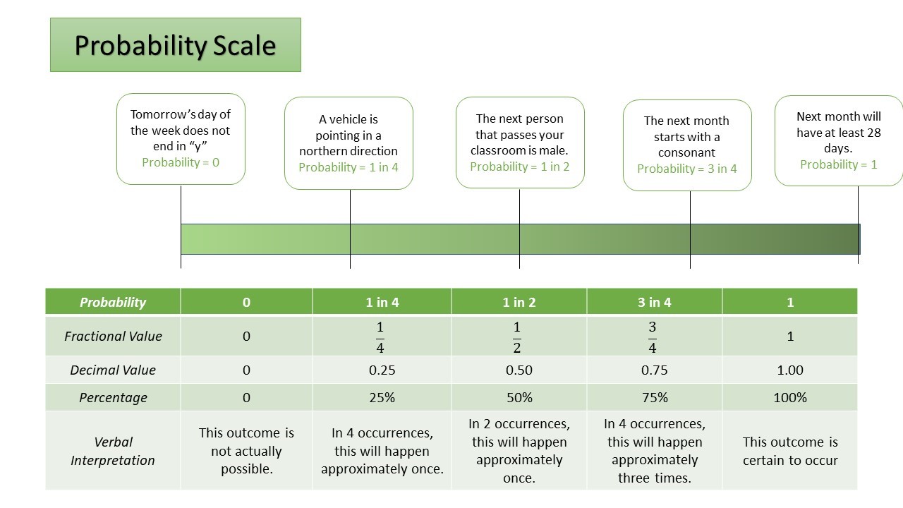
Probability is a specific type of ratio that allows the comparison of specific outcomes with the entire group of outcomes. We see probability expressed in three ways: as a fraction ranging from 0 to 1, as a decimal ranging from 0 to 1, and as a percentage ranging from 0% to 100%. All three of these expressions allow us to see a part and a whole, even if in the case of decimals and percentages where the whole is adjusted to be a multiple of ten. These different expressions can be seen in the Probability Scale below.
We have two main ways that we think about probability. One is what is called a theoretical model. In the theoretical model, probabilities are driven by expectations of what we know. One classical example of a theoretical model is a coin flip where we know that there are two specific outcomes, or thinking about the months of the year from the probability scale. The second model is called an empirical model, and it is based on directly counting the occurrences of outcomes from events that have occurred. The empirical model is useful when the event being studied does not happen regularly. The process of selecting objects to model a process is called a probability experiment. A probability experiment offers a way to explore different outcomes. We can manually calculate the outcomes of a probability experiment, or use a tool like a simulator to help us understand a situation that is represented in a statement. Our choice to do this depends on the outcome or event that we might be looking at.
Both theoretical probability and empirical probabilities have similar building blocks. The sample space is the collection of all possible outcomes. An event consists of one or more outcomes. The probability is a ratio of the specific event of interest over the total number of outcomes. In this module, while we recognize the importance of understanding the underlying formulas for probability, we rely on simulations to develop skills that link initial statements of probability and the outcomes of experiments.
Exploration 9.7.1.
Consider the statement: “A student feels safe to be themselves at school.”What outcomes are possible?
Are there reasons that might cause students to feel unsafe about being themselves?
Do you think a student being themselves could make another student uncomfortable? Why or why not?
The possible outcomes are {a student feels safe, a student does not feel safe}, and that makes sense. The probability of a student feeling safe to be themselves will result in 1 out of 2 outcomes, but can we reliably predict which outcome we see? Ideally, students feeling safe to be themselves at school should be the only outcome we expect to see. In reality, we find that students do not feel safe to be themselves at school for any number of reasons. Consider the following quote: “The teachers … they thought we were selling weed in school, they thought that me and her were both selling weed ‘cause like, the way we were dressing, ‘cause we were the only girls at that middle school that dressed like boys. So it was like 'now we’re bad'.” (non-gender conforming youth from Arizona) [9.12.168]. In this quote, the student was exposed to a negative experience, accusations of illegal activity, because of choices associated with how they chose to express who they believed themself to be.
Making Sense: Think back to your experiences in school. Identify if there were similar incidents to the incident described above in your community. Do you think that how people were seen by others influenced their behavior, meaning if a label was applied to a person did they adapt to the label? Or do you think that the person stayed the same?
The second type of probability that we use is the empirical model. This comes from raw data. We tend to see this in the form of tables with numeric values, instead of the summary statistics. The basic use of the empirical model is very similar to the ideas from theoretical probability, and when we think about how to make sense of data from a table of data we think about what the theoretical model might have to look like.
Exploration 9.7.2.
The data in the table below is taken from a report by the American Civil Rights Union (ACLU) [9.12.157]. The report states that students in these three states have the same general probability of being arrested per 10,000 students. For many states being arrested as a form of school discipline aligns with zero tolerance offenses that qualify for expulsion. For this reason, we may make a reasonable assumption that students may not be arrested multiple times as a form of school discipline.Our first step to exploring the claim in the document is to think about the probability that we want to build. If you are a student going to school, when it comes to being arrested, you either get arrested at school or you don’t get arrested at school. So we have two groups of students, those that get arrested and those that don’t get arrested. We also happen to know about the number of students that get arrested, as well as how many students there are. This means that we have everything we need.
To find the probability of being arrested, we find the ratio of arrests to students for each state. For this example, we will model with Missouri and you can test your ideas on Arkansas and Rhode Island.
We can reduce this to a decimal figure, as finding common factors or a reduced form fraction is highly unlikely. This yields approximately 0.001625.Now we want to know how this fits with thinking about the probability of being arrested per 10,000 students. In other words, if the probability of getting arrested is 0.001625, this is about 0.1625%; how many arrests would that be among 10,000 students? We use this previously calculated value and solve an equation, to find a value out of 10000:
Solving this equation gives a value of 16 whole students in Missouri per 10000 based on the overall probability. The report claims that you have the same probability per 10000 in all three states. Can you verify the claim?
Those are the basics of probability. We can use these basic ideas of probability to help us build more complex models that can help us build more complex structures.
Subsection 9.7.1 The complement
The first of these complex structures is the complement. We generally define the probability of a complement as the probability of an event of interest not happening. In Exploration 9.7.2, we identified that there were two specific groups: students that got arrested and students that did not get arrested. The probability of not getting arrested can be found in two ways: either by calculating it directly or by subtracting the opposite event from 1.
Example 9.7.2.
To find the probability of not getting arrested in school in Missouri, we know that there are 915,033 total students, and we also know that only 1,487 were arrested. So we know that the rest of the students were not arrested. So, we can subtract the arrested students from the total students to find the not arrested students, which gives us 913,546 students that were not arrested. We then find the ratio of not arrested students to total students: 913,546/915,033=0.998375, or around 99.3875%.
We can also find this by using the fact that we know the probability of getting arrested. We start with the group of all students (1), and then we subtract out the group that represents getting arrested: 1 - 0.001625=0.998375, or 99.8375%.
We get the same mathematical answers from calculating the complement using either method. It is important to understand both methods because we have to think about the different types of information that we might have available. What is something that we notice in this scenario? Can a person be both arrested and not arrested at the same time? That leads us to our second special scenario.
Subsection 9.7.2 Mutually exclusive events
One consideration in probability is the consideration of if events can occur at the same time. One example of events that cannot occur at the same time are an event and its complement, so thinking about our prior example a student cannot be both arrested and not arrested at the same time. This is an example of mutually exclusive events. But when we start to think about more complicated events, like can you be a specific race and be suspended from school, the events become more complicated. Understanding if events are mutually exclusive or not, allows for better and more accurate methods of calculating probabilities. Having more accurate probability calculations can help us make more informed judgments about issues.
Example 9.7.3.
Determine if you think the following event pairs are mutually exclusive or not. Explain to yourself why you think they are or are not mutually exclusive. What information did you use to make your decisions?
Event Pair A: Being Black and Getting suspended from school
Event Pair B: Being truant and Having regular school attendance
Event Pair C: Making good grades and Being disciplined in school
Following up: Based on models we have looked at, we realize that being Black and getting suspended can happen together, so those events are not mutually exclusive. When I know that being truant means not attending school regularly, I realize that the events in Event pair B are complements and have to be mutually exclusive. Event pair C is the most difficult to really take apart. Common sense-wise and experience-wise it seems like maybe the people who got good grades didn’t get in real trouble at school, but then again there is no reason why they couldn’t get into trouble. This means that they have to be not mutually exclusive events.
Subsection 9.7.3 Independent Events
There is another way to think about multiple outcomes, and this happens when the events happen independently. In independent events, two separate events happen that have the same underlying probability, or at least we would like to think that they should (refer to Exploration 9.7.1 for more detail). This is the crux of many arguments about school discipline. For an event to be independent, the underlying probability of the event should be the same across all subgroups. Consider an event like being enrolled in the reduced lunch program. If the probability of enrollment is approximately the same for all racial subgroups, then being in the reduced lunch group and the being in racial subgroups are independent. From your experience, do you think this is always the case? Feel free to use any relevant examples.
Let’s look at an example of how the math of independence works. For calculations, we assume that individual events are independent.