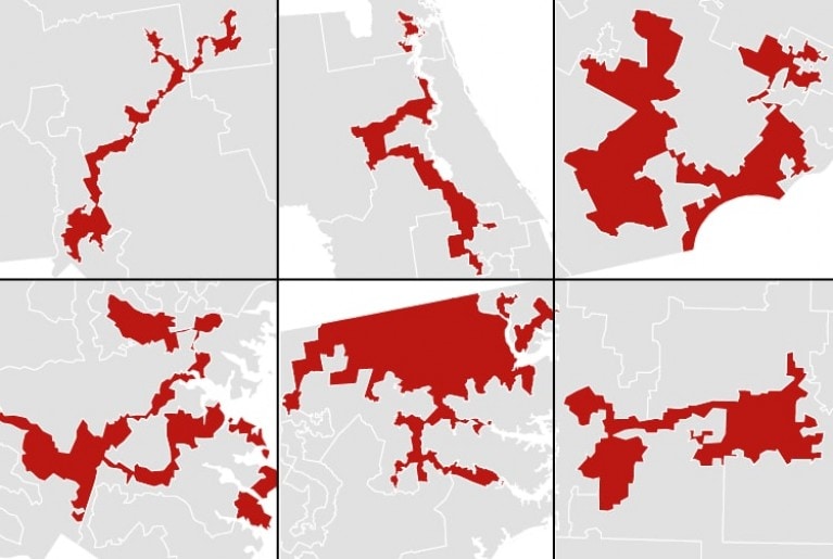
As mentioned in the chapter overview, the term “gerrymander” originated from a critique of an unusual district shape in Massachusetts in 1812. Since then, many discussions about manipulation of district boundaries have focused on the shapes of the districts. Take a look at the shapes of some recent congressional districts, as presented in a Washington Post article [4.12.42]:
Figure4.5.1.Collection of images of 6 different districts. The districts have squiggly borders and narrow regions spread over a wide area. This is only a sampling of bizarre district shapes; in fact, some people even created a computer font called Ugly Gerry (see [4.12.39]) using real district shapes!
But what is compactness, and why should we care about districts having nice shapes? Compactness is a quantitative measure of a district’s shape and how tightly packed, or compact, the region is. Remember that the function of a political district is to elect someone that represents the people, needs, and interests of an area. A district over a more compact area is likely to include towns and communities with similar interests, while a district that zigs and zags across a state is more likely to intentionally exclude certain groups of people and connect regions with different local interests. In fact, most states include language emphasizing the importance of “compactness” of their districts but lack a definition or a way to measure this characteristic.
Motivating Questions: To what extent can or should we use the shapes of districts to determine a potential gerrymander? Can we agree on an accepted way to measure compactness since many states specifically include it as a consideration for district plans?
Subsection4.5.1Packing and Cracking: How drawing lines can change outcomes
Why might districts be drawn in squiggly shapes stretching over large areas? How can the shape of a district matter if we count all votes equally? Consider this brief introduction to two key terms: packing and cracking.
Introduces packing and cracking. Images show cartoon examples of plans that use these techniques to achieve desired outcomes.Figure4.5.2.TedEd video introducing packing and cracking.
Subsection4.5.2Three Ways to Measure Compactness of a District
Remark4.5.3.
There are many different mathematical and geometric approaches for measuring the compactness of a shape. It is important to note that these measures are based entirely on district shapes and do not factor in geography, racial demographics, political party affiliation, or election results. While the shape of a district alone is not indicative of gerrymandering, it can be worthwhile to consider as one potential indicator. We examine a few measures here.
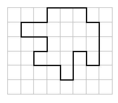
To allow for more straighforward computations, we work in square grids in this section, noting that this is a simplification from real-life applications. We start with our square grid and a district plan drawn on the grid:
Figure4.5.4.Square grid with district plan.
We defined compactness above as a measure of how tightly packed a district is. The most compact district, then, is one that is as tightly packed as possible. If we are constructing our districts from squares in the grid, what shape would be as tightly packed as possible? We would want smooth edges, without any parts sticking out, so we might try to arrange our squares into a rectangular region. But a long, skinny rectangle would not be considered as tightly packed as possible: we could tighten it up even more by getting the side lengths to all be the same. Our most compact shape, then, is a square.
The first measure of compactness we discuss, the Polsy-Popper measure, is found by comparing the shape of a given district to the “ideal” shape, a square - more specifically, a square that has the same perimeter as our district.
Definition4.5.5.
The Polsby-Popper score is a ratio that compares the area of a district to the area of a square with the same perimeter as the district. Thus we have
\begin{equation*}
PP =\displaystyle\frac{\text{Area of district}}{\text{Area of a square with the same perimeter as the district}} \text{.}
\end{equation*}
In the following example, we calculate the Polsby-Popper score for the district above.
Omitting units and simply counting, we note the area of the district is \(18\) and its perimeter is \(26\text{.}\) Since all sides must be equal in length in a square, any square that has perimeter \(26\) must have sides of length \(\frac{26}{4}\) or \(\frac{13}{2} \text{.}\) Therefore the area of this square would be \(\left ( \frac{13}{2} \right )^2 = \frac{169}{4}\text{.}\) Now we find the ratio: \(PP = \frac{18}{(169/4)}=\frac{72}{169} \approx 0.426.\)
Our second measure of compactness, the Reock score, again compares the given district shape to a square. However, instead of using a square with the same perimeter as the district, the Reock score compares to a minimum-bounding square, which is the smallest square that fully contains the district.
Definition4.5.7.
The Reock score is a ratio that compares the district’s shape to the minimum-bounding square, the smallest square that fully contains the district. We have
\begin{equation*}
R =\displaystyle\frac{\text{Area of district}}{\text{Area of the smallest square containing the district}} \text{.}
\end{equation*}
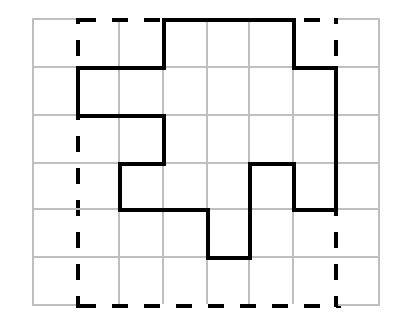
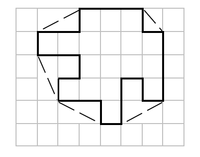
In the image below, we show the district plan together with the smallest square containing the district.
Figure4.5.8.District plan with minimum-bounding square. The minimum-bounding square is outlined in dashed line. Because the district is 6 squares wide at its widest point, the minimum-bounding square is 6 units by 6 units.
In the next example, we calculate the Reock score for the district above.
Omitting units and simply counting, we note the area of the district is \(18\) and area of the smallest square that contains the district is \(36\text{.}\) In this case, we have \(R = \frac{18}{36}=\frac{1}{2}=0.5\text{.}\)
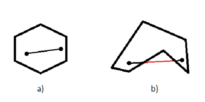
Finally, the Convex Hull score is a ratio that measures how “convex” a district shape is. In geometry, a convex shape is one in which any two points in the interior of the shape can be connected by a straight line that stays inside the shape. If there is any pair of interior points connected by a straight line that partially falls outside of the shape, then the shape is known as concave. The picture below shows an example of a convex shape (image a) versus concave shape (image b):
Figure4.5.10.Convex and concave shapes.
The convex hull of a shape is the original shape together with the minimum additional area needed to make it convex. To visualize the convex hull, imagine placing a rubber band tightly around the perimeter of the shape. If the shape is a square, or a rectangle, the rubber band will fit exactly along the edges of the shape. If the shape is not rectangular, the rubber band will stretch across any gaps created between corners of the shape. This region enclosed by the rubber band is the convex hull. The picture below shows our district together with its convex hull:
Figure4.5.11.District plan with convex hull. The convex hull is outlined in dashed line, and can be thought of like a rubber band stretched around the district border.
Definition4.5.12.
The Convex Hull score is a ratio that compares the district’s shape to its convex hull. It is defined as
\begin{equation*}
CH =\displaystyle\frac{\textnormal{Area of district}}{\textnormal{Area of convex hull of district}}\text{.}
\end{equation*}
In the following example, we compute the Convex Hull score for the given district.
Find the Convex Hull score for the district above. Hint.
The convex hull around the district is outlined in a dashed line. Find the area of this region by combining the area of the enclosed squares with the areas of the triangular regions formed.
Omitting units and simply counting, we note the area of the district is \(18\text{.}\) The area of the convex hull that contains the district is found in pieces, combining the area of the squares with the areas of the triangular regions formed. For area of the convex hull we get \(20 + 4 + 0.5\text{.}\) This yields \(CH = \frac{18}{24.5} \approx 0.74 \)
Remark4.5.14.
The actual formulas for these scores (based in the real world rather than districts composed of squares) vary slightly from those we use here. In particular, the “ideal” compact shape used for comparison in the first two measures is a circle. In the Polsby-Popper ratio, the ideal shape is a circle with the same perimeter (circumference) as the district. In the Reock ratio, the ideal shape is the minimum-bounding circle, which is the smallest circle containing the district. Our definitions and compactness scores are consistent with the formal scores and allow for more straightforward computations.
Subsection4.5.3Compactness Criteria
In these three measures, compactness is a geometric measure that compares the area of a district to some “ideal” compact shape. In each case we consider, the compactness score is a number between 0 and 1 that measures the compactness of the shape relative to the ideal. Districts closeWindow() in shape to the ideal shape (more compact) have scores closeWindow()r to 1, while those less compact (farther from the ideal) score closeWindow()r to 0. When a district has much greater perimeter than we would expect for the region’s area (as happens when the shape has long, skinny pieces branching off or strung together), we may suspect gerrymandering. At this time, 37 states include a compactness requirement for state legislative districts, and 18 establish similar requirements for congressional districts. However, there is no universal measure, and different states have different laws that regulate compactness. In Idaho the redistricting commission is expected to “avoid drawing distorted boundaries” [4.12.41], while in other states with extensive coastlines (such as Maryland) this is impossible. In fact, most states do not provide details on compactness measures but adopt a “you know it when you see it” approach in determinations.
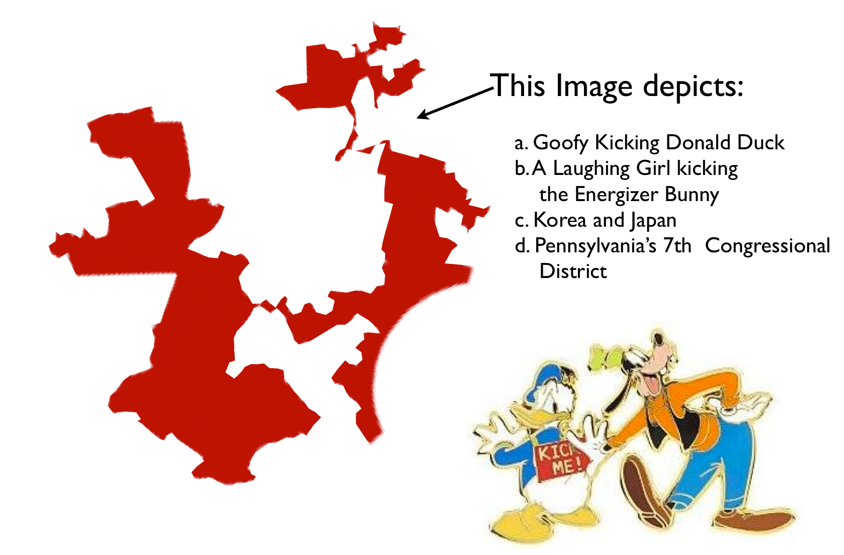
Compactness in the Courts: Pennsylvania’s 7th congressional district adopted in 2011 (shown below) has been widely cited as an example of a district that is far from compact as a result of gerrymandering. In 2018, the state’s Supreme Court ruled this (and the rest of the district plan) to be an unconstitutional gerrymander, and required the state to create a new map. [4.12.35]
Figure4.5.15.PA 7th district, 2011 (“Goofy kicking Donald Duck”). For more on this district, see [4.12.40].
Among mathematicians and political scientists, the debate about best measures of compactness continues, but consensus has arisen around a few guiding principles:
There is no number threshold for a district being deemed “compact” - the numbers are used in comparison, not for their standalone values.
Compactness measures should be used across an entire districting plan, not just a single district.
Comparisons should be made between districts and plans within the same state, and not across different states as each state’s geography is unique.
Compactness tests should measure the shape and not the size of the district.
Multiple compactness tests should be used whenever possible.
Compactness tests should not be the sole factor used to judge district plans.
We have repeatedly mentioned that geometry cannot be a sole measure of fairness, though many states do require it to be a consideration in redistricting. There are many different factors possibly contributing to a district’s shape, as summarized in the following quote:
"But sometimes boundaries that look odd at first glance just follow a natural geographic feature, like a river or a mountain range. Or they could be necessary to unite communities that live in different areas but share similar representational needs, like communities of color that have been subject to residential discrimination. Other times, odd boundaries are very much the product of gerrymandering. [...] The reality is that visual inspection can be a helpful, but ultimately very incomplete, analysis. It is a good first test that can help identify where a deeper dive is needed. In other words, don’t judge a book by its cover." [4.12.32]
The Brennan Center has gathered several examples of situations like these in this useful analysis: Don’t judge a district by its shape (opens new tab) 1 . In fact, as the article points out, it is possible for a compact shape to be the result of a gerrymander too! In the following sections, we explore issues of fairness that go beyond geometry.