Understanding data

Section 7.5 Understanding data

We have two large data sets, adapted from the Stanford Open Policing Project [7.10.124], giving information on vehicular stops in Hartford, CT and Philadelphia, PA between April 1, 2014 and September 29, 2016. Anyone can access these data sets at https://openpolicing.stanford.edu. Below are the first two rows from the Philadelphia data set.\\

Table 7.5.1.

date	time	age	race	sex	searchfrisk	contraband	arrest
2014-04-01	0:00:00	20	white	male	FALSE	NA	FALSE
2014-04-01	0:04:00	33	black	male	FALSE	NA	FALSE

We call each row an observational unit or observation. In this case, each observation is one vehicular stop. Each column is called a variable; here we have 8 variables. First, the date and time of the stop are provided. The next three variables give the age, race, and sex of the driver of the vehicle.

The searchfrisk variable is TRUE if the vehicle was searched or the driver was frisked and FALSE otherwise. If either the vehicle was searched or the driver was frisked, contraband is TRUE if an item was found which was illegal for the driver to possess and FALSE otherwise. If no search or frisk was conducted, contraband cannot be found, so NA (for ``not available'') is written. Finally, the driver is either arrested (TRUE) or not arrested (FALSE).

The age variable is a numerical variable since the response is a number and it makes sense to perform arithmetic operations on these numbers, such as addition, subtraction, or computing averages. The last five variables are not numerical. Since the responses to these variables fall into different categories, these are called categorical variables. We won't be analyzing the date and time variables, but whether they are considered numerical or categorical depends on the situation.

Subsection 7.5.1 Summarizing Data

Subsubsection 7.5.1.1 Numerical data

Suppose we are given the following values of a numerical variable:

\begin{equation*} [2,10,3,6,8,3,4,5,2,3,5,6,1,7,9,8,10,8.] \end{equation*}

These values could represent the cost of 18 different taxi rides or 18 students' scores on a quiz or the number of petals on 18 different flowers.

We often want to find the ``center'' or ``middle'' of the values. To compute the mean, we simply add up the values and divide the total by the number of values. In this case, we get

\begin{equation*} \frac{2+10+3+6+8+3+4+5+2+3+5+6+1+7+9+8+10+8}{18}=\frac{100}{18}\approx 5.56. \end{equation*}

We could say that, on average, each taxi ride cost $5.56, or that the average score on the quiz was 5.56. But sometimes the mean can hide useful information. Suppose we have a class of 10 students and one student has 10 cookies, while the other 9 students have 0 cookies. The mean number of cookies each student has is

\begin{equation*} \frac{10+0+0+0+0+0+0+0+0+0}{10}=1. \end{equation*}

So, on average, each student has 1 cookie. But the ``average student'' definitely does not have one cookie--in fact, almost all of the students have 0 cookies!

The median is the middle value once the data is sorted (if there is an even number of values, the median is the mean of the two middle values). For our initial example, we first sort the data:

\begin{equation*} [1,2,2,3,3,3,4,5,5,6,6,7,8,8,8,9,10,10.] \end{equation*}

Since there is an even number of values, we take the mean of the two values in the middle, which are 5 and 6. Hence the median is $\frac{5+6}{2}=5.5\text{.}$ Notice that half of the values are less than the median and half are greater.

But what if we want to know more about the data we have than just the mean and median? We can create a histogram. The histogram below provides one way to visualize the data from our initial example.

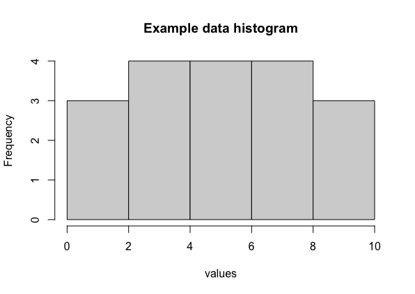
On the $x$-axis, we've grouped our values into intervals--the leftmost interval goes from 0 to 2, inclusive. The height of the bar in this interval (called the frequency) is 3, since there are three values ($1,2,2$) in our data in this interval. The next interval goes from 2 to 4. The interval includes 4 but it does not include 2. The frequency here is 4, because our data included three 3s and one 4. The third interval goes from 4 to 6, and again includes its upper endpoint, 6, but not its lower endpoint, 4. The frequency here is 4, because our data included two 5s and two 6s. The final two intervals are from 6 to 8 (including 8 but not 6) and 8 to 10 (including 10 but not 8). The frequencies in the last two intervals are 4 and 3, respectively.

Let us apply these ideas to the age variable from the Hartford data. Since there 9630 stops recorded in this data set, computing the mean and median by hand would take a long time! Instead, we'll use R, a programming language heavily used in statistics. The functions mean and median give the mean and median of the variable age, while hist creates the histogram. Just hit "Evaluate R"" below each block of code to see the results!

Subsubsection 7.5.1.2 Categorical data

If our data is categorical, none of the previous methods work--we can't take averages or sort the data from least to greatest. Nor can we create intervals and use these to make histograms.

However, there are still a couple things we can do! We can summarize data in a table or make a bar chart.

Consider the sex variable from the Hartford data set. We first make a table in R

From this table, we can see exactly how many of the stopped drivers were male and female. Then, we can use these numbers to determine the proportion of stopped drivers who were female by dividing the number of females (which we just found in the table) by the total number of stops (which we know is 9630). We can get a visual representation of this same data by making a bar chart.

Subsection 7.5.2 Proportions

Subsubsection 7.5.2.1 Are there more traffic stops in Hartford or Philadelphia?

This question seems easy to answer. We can determine the number of stops in each city between April 1, 2014 and September 29, 2016 using the nrow function.

There were a lot more stops in Philadelphia (678,445) than in Hartford (9630)! In fact, there were

\begin{equation*} \frac{678445}{9630}\approx 70 \end{equation*}

times as many traffic stops in Philadelphia than in Hartford. Does this mean people in Philadelphia are worse drivers or commit more crime? Not necessarily--there are many more people in Philadelphia, so it makes sense that there are more traffic stops. Using data from the U.S. Census Bureau, we see that Philadelphia had approximately 1,555,000 people in 2015 and Hartford had 125,000 [7.10.125], [7.10.126]. Therefore, there were

\begin{equation*} \frac{155000}{125000}\approx 12.4 \end{equation*}

times as many people in Philadelphia than in Hartford.

Well, that's interesting. Philadelphia had about 13 times the population, but 70 times the number of traffic stops as Hartford. These data show us that, there were many more traffic stops in Philadelphia than in Hartford in this time frame, even when we control for population. Unfortunately, the data cannot tell us why this is the case. Further research, with the help of experts in policing, history, crime, and a slew of other subjects may help us.

Subsubsection 7.5.2.2 Are Black drivers stopped more often than drivers of other races?

Now let's look at the racial makeup of the stopped drivers in each city. The data here isn't perfect; there are only six possible options for race: asian/pacific islander, black, hispanic, white, other, and unknown. Many, many people do not fit neatly into one of these categories, but we do what we can with the data we have. We use the table function to get the numbers we want.

Using these tables and the total number of stops in each city, we see that

\begin{equation*} \frac{3589}{9630}\approx 37.3\% \textrm{ and } \frac{435548}{678445}\approx 64.2\% \end{equation*}

of the drivers stopped were Black in Hartford and Philadelphia, respectively. We now compare these percentages to 2015 population data from the US Census Bureau. For Hartford, 37.3\% of the drivers stopped were Black and 38\% of the population was Black--these numbers seem to indicate that Black drivers were not stopped more frequently than drivers of other races [7.10.125]. In Philadelphia, however, 64.2\% of the drivers stopped were Black while only 42.4\% of the population was Black [7.10.126]. It seems as though Black drivers were disproportionately stopped in Philadelphia during this time. Let's use the data on searches, contraband, and arrests to give us more insight.