
Section 6.7 Correlation
Our final mathematical topic for this module will be correlation. When we looked at the background of payday lenders, we talked about the fact that they are more likely to be located in majority Black and Latinx neighborhoods. We'll look at analyzing this mathematically through the lens of correlation.
Subsection 6.7.1 Defining the Correlation
Suppose we have two sets of numbers:
If someone told you that the next number in the first set was 30, what would you expect the next number in the second set to be? You would probably guess 60, because there's a clear pattern here - the number in the second series is always exactly double the corresponding number in the first series.
In practice, when we look at two sets of data, the relationship between them is rarely this exact. For example, look at these two sets of data:
The values in the second set are just a little bit off from two times as much as the first set. If someone told you the next number in the first set was 30, though, you would still probably expect the next number in the second set to be approximately 60 - maybe not exactly 60, but something closeWindow(). Even though one number doesn't exactly predict the other, it comes pretty closeWindow().
The correlation is a way of measuring how closeWindow()ly one set of numbers predict another. The correlation gives a number between 1 and -1. A correlation of 0 means that there is absolutely no relationship between the two sets of numbers - when one changes, you can't predict what will happen to the other. A correlation of 1 means that there is a perfect relationship between the numbers - when the values in the first data set increase, the values in the second data set increases in a way that exactly corresponds. Our first two sets of numbers would have a correlation of 1. Our second pair would have a correlation closeWindow() to 1, but not exactly 1. A correlation of -1 also indicates a perfect relationship, but when one of the values in one set increases, the values in the second set will decrease in a way that exactly corresponds. So the pattern is still perfect, but it works in reverse.
Computing the correlation is tricky. We'll go through the process of computing it, which takes multiple steps, but in general we'll do it using software. The R programming language lets us easily find the correlation between two sets of numbers. Here, you'll see the two data sets we looked at above. The cor function in R calculates the correlation between two sets of numbers - hit "Evaluate R" to calculate. You can try different values in the exercise below - just hit "Evaluate R" to find the correlation. You'll see that when we look at the first pair of data sets, the correlation is exactly 1:
If we look at the second pair, though, the correlation is a little less than 1. 0.9812022 is still very closeWindow() to 1, though, because these numbers still mostly fit the pattern - just not perfectly.If we have numbers that are completely unrelated, though - where there is no pattern between how much one increases by and the other - we'll see very low correlation:
Subsection 6.7.2 Computing Correlation
Computing the correlation is a little complicated, and is easiest done in multiple steps. While it's not crucial that you can go through all of these steps on your own, we'll explain how the correlation is defined to help understand why it computes how related two sets of data are.
Correlation.
If we have two sets of data \(x = {x_1,x_2,\ldots,x_n}\) and \(y = {y_1,y_2,\ldots,y_n}\) with the same number of values, the correlation is
where \(\overline{x}\) and \(\overline{y}\) are the means of \(x\) and \(y\text{,}\) and \(s_x\) and \(s_y\) are the sample standard deviations of \(x\) and \(y\text{.}\)
You can compute the mean by adding up all the values and dividing by \(n\text{.}\)
You can compute the sample standard deviation by subtracting the mean from each value, squaring that, adding them all up, dividing by \((n-1)\text{,}\) and taking the square root.
This is a pretty complicated formula, but it turns out it's pretty easy to break it down into steps.
Compute the means \(\overline{x}\) and \(\overline{y}\text{.}\)
Compute the sample standard deviations \(s_x\) and \(s_y\text{.}\)
Subtract the mean \(\overline{x}\) from each value in \(x\text{,}\) and the mean \(\overline{y}\) from each value in \(y\text{.}\)
Multiply the corresponding differences from \(x\) and \(y\) together.
Add them all up.
Divide the whole thing by \((n-1)s_x s_y\text{.}\)
Let's see how this works with the second data set above:
First we'll compute the means and sample standard deviations of each data set:
Now that we have all of these, let's get down to the work of calculating the correlation. Our next step is to subtract the mean from each data value in \(x\) and \(y\text{:}\)
Now we'll multiply each corresponding pair together:
Now we'll add up all the values:
And finally, we divide by \((n-1)s_x s_y\text{.}\)
This is the same value we got from R above, up to 3 decimal places (the difference comes because we rounded \(s_x\) and \(s_y\))
Subsection 6.7.3 Using Correlation
Ok, so we've defined this correlation, which tells us how one set of numbers is related to another. But why does it matter?
An old adage says that "correlation does not imply causation," meaning that just because two things are correlated doesn't mean that change to one causes the change in another. Two things could be correlated that are completely unrelated. For example, there is a strong correlation (0.9039) between the number of bee colonies in the US and the divorce rate in South Carolina:
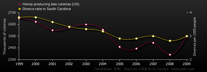
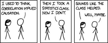
Does this mean that bees are breaking up marriages in South Carolina, or that new divorcees are running out to start beekeeping? Of course not (or at least, probably not). We don't have any other reason to believe that one of these variables is causing the other. But when there is some reason why we might believe that one thing is causing another, the correlation can give us evidence to support that theory.
For example, because of the legacy of systemic racism and intentional exclusion of Black Americans from the financial system, we could theorize that there are fewer banks - and more payday lenders - in majority Black neighborhoods. We could use correlation to see if there is evidence for this theory - by looking at the racial makeup of a neighborhood and seeing if there is a correlation with the number of financial institutions. This doesn't prove that banks are intentionally avoiding Black neighborhoods (though other evidence may support that claim) - it just provides evidence to support that theory.